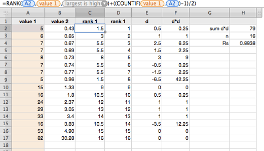
Michaela is doing a biostatistics paper, and today she was working on calculating Spearman’s Rank Correlation. While she was doing this by hand, I set about doing it in Numbers.
The tricky part was the ranking, as the textbook says to give equal ranking items the ‘average of the ranks’ they would have if unique, thus the values {10, 11, 11, 12} have the rank’s {1, 2.5, 2.5, 4}. The RANK function in Numbers gives nth equals ranking (thus giving {1, 2, 2, 4} for the prior data).
To calculate Spearman’s Rank for value A2 from column A use (in C2 for example):
=RANK(A2,A,1)+((COUNTIF(A,A2)-1)/2)
Pulling the formula down for all values in A (giving the ranks of A in column C). Do again for the second of the paired values in B (into column D). You then can calculate d and thus calculate d2 in their own columns and finally get Σd__2. With n in cell H3 and Σd__2 in cell H2 you can pop this into a cell:
=1-((6*H2)/(POWER(H3,3)-H3))
and get your r__s
Looking at the Wikipedia article, it has a single line Excel formula, but the Numbers RANK function is not as complete as Excel’s, so you can’t use it. The formula also uses the CORREL function, but that is a linear regression, not the Spearman’s regression, so it’s not much use here either. Thus it seems you need an ugly table like this it after all:

This all applies to Numbers ‘09.
